Beat the Bookie: Predicting EPL Matches with ML
A UCL group project where we tried to out-predict bookmakers on 10 Premier League matches using XGBoost, SVM, K-Means, and a DNN. Spoiler: we mostly predicted home wins.
For a machine learning coursework at UCL, my team and I were given a straightforward-sounding challenge: predict the outcomes of 10 Premier League matches scheduled for 1 February 2025. Win, lose, or draw — for each game. The project was called Beat the Bookie, and the benchmark we were trying to clear was the accuracy of professional bookmakers, which sits around 53%.
We ended up at 54% with our best model. Not a revolution, but a genuine beat. Here’s what we actually did to get there.
The full code is on GitHub if you want to dig in.
The Problem
Predicting football results is a three-class classification problem: Home Win (H), Away Win (A), or Draw (D). The baseline for random guessing is 33%, so the real question isn’t whether you can beat a coin flip — it’s whether you can get meaningfully close to what bookmakers with decades of data and entire teams of analysts produce.
The 10 matches we had to predict were all played on the same day, which meant we couldn’t use live or in-game data. Everything had to come from historical match records and whatever external data we could scrape.
Data and Feature Engineering
The provided training dataset covered historical EPL matches, but raw match data alone isn’t very predictive. Goals, shots, cards — these tell you what happened, not how a team is likely to perform next. Most of our effort went into engineering features that were more forward-looking.
We pulled external data from three sources via web scraping: FBREF for referee statistics and league standings, TransferMarkt for team market values, and WhoScored for possession averages and set-piece efficiency.
Missing values were a genuine problem — possession percentages and penalty efficiency weren’t available for every season. Rather than filling in means, we used model-based imputation: Random Forest Regression for set-piece and penalty efficiency, and XGBoost Regressor for market values and possession. The idea was to use correlated features to estimate missing values rather than just guess.
What actually predicted outcomes
One of the first things we looked at was goal rate — the proportion of shots that resulted in goals, defined as FTHG / HS for the home team. The scatter plot below makes the relationship fairly clear: teams with a higher goal rate tend to win more at home.
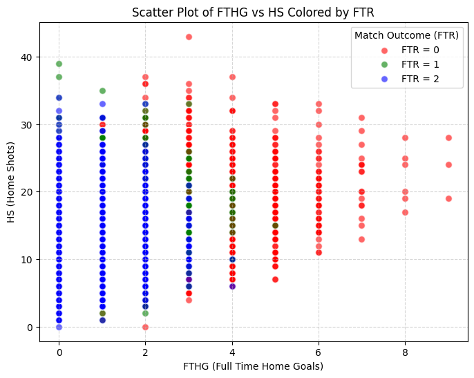
This gave us a useful derived feature on top of the raw shot counts already in the dataset.
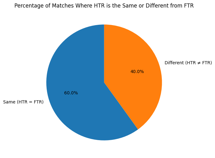
Half-time results turned out to be another strong signal. Around 60% of matches share the same outcome at half-time and full-time, which means how a team typically performs in the first half is genuinely informative about the final result.
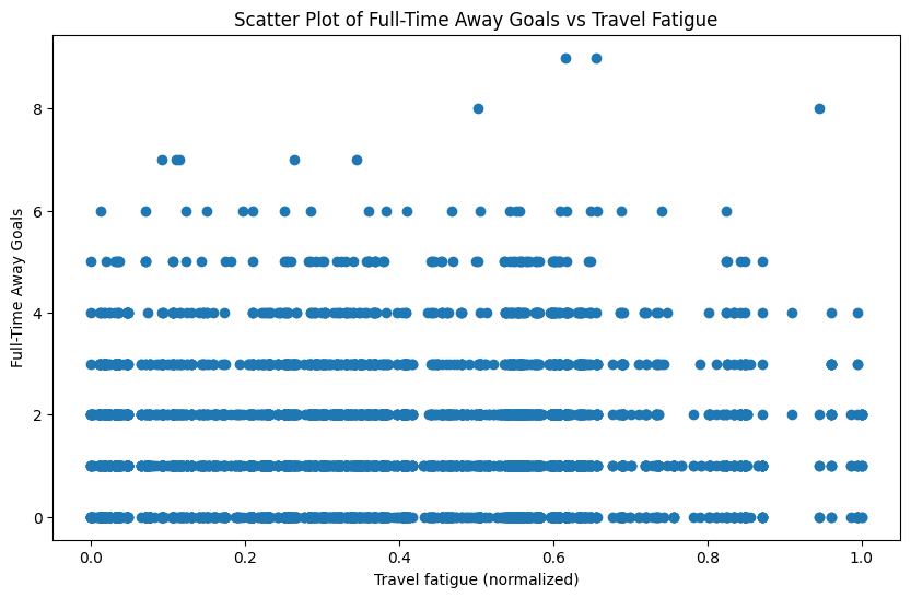
Beyond in-game statistics, environmental factors had a measurable effect. Travel distance for the away team — used as a proxy for fatigue — showed a clear relationship with home team performance. Bigger travel distance, better home result on average.
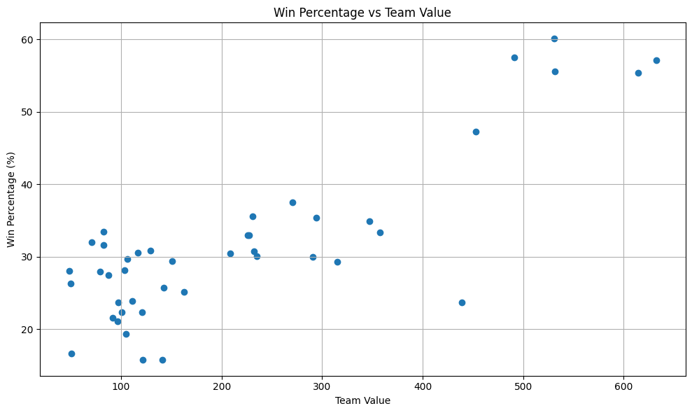
We also incorporated team market values from TransferMarkt, on the intuition that wealthier squads generally win more. This held up well empirically.
A few other findings from the EDA worth noting: yellow cards showed almost no predictive signal and were effectively dropped. Red cards had a slight effect but nothing dramatic. Possession was useful but weaker than you might expect.
The final feature set
In total, we engineered 13 features on top of what the dataset provided. A few of the more interesting ones:
14-Day Match Density — the number of games a team played in the 14 days before the match, across all competitions. A proxy for fatigue and squad rotation pressure.
Referee Strictness — (3 × red cards + yellow cards) / total matches officiated. Red cards are weighted higher since they directly change the game.
Team Form Points — rolling sum of points over the last 10 matches (W=3, D=1, L=0), plus the difference in form between home and away teams as a separate feature. Comparative features like this tended to matter more than absolute values alone.
Head-to-head win rate — historical record between the two specific teams, not just overall recent form.
The Models
We tested four models. The brief required multiple approaches, but comparing them turned out to be genuinely instructive — particularly around the draw prediction problem.
XGBoost
Our main model. XGBoost is a gradient-boosted decision tree ensemble: it builds trees sequentially, each one correcting the errors of the previous one. It handles missing values natively, doesn’t require feature scaling, and performs well on tabular data without much hand-holding.
We used DART as the booster (Dropouts meet Multiple Additive Regression Trees), which applies dropout-style regularisation to the ensemble to reduce overfitting, combined with early stopping on the validation set. Learning rate: 0.001, dropout rate: 0.1.
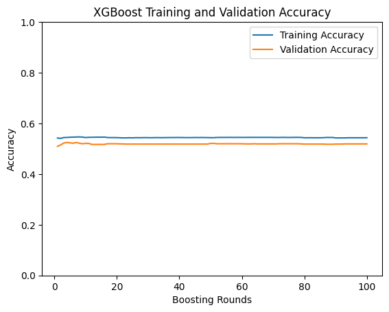
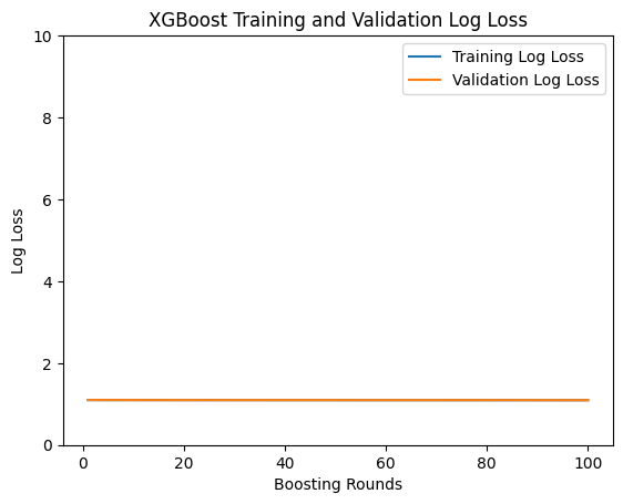
Training and validation accuracy tracked closely throughout, and both loss curves converged downward — a clean result with no obvious overfitting. Final accuracy: 54%. Strong F1 on Home Win and Away Win, but it never once predicted a draw, which is a meaningful limitation we’ll come back to.
Deep Neural Network
A multilayer perceptron with several hidden layers. The first run was revealing: 86% training accuracy with only 47% validation accuracy, and a validation loss trending upward. Classic overfitting.
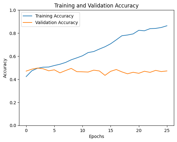
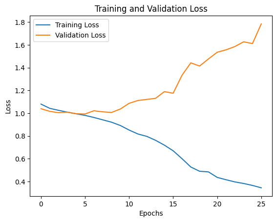
After dropping the learning rate to 0.00005, increasing dropout to 0.5, and adding L2 regularisation (λ=0.01), the gap narrowed considerably. Both loss curves trended downward together.
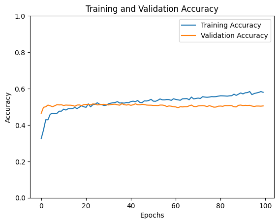
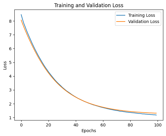
Final accuracy: ~50%. Better at predicting draws than XGBoost, but lower overall. The before/after comparison here is a clean illustration of what overfitting looks like and what regularisation does to fix it.
SVM
Support Vector Machines find the hyperplane that maximally separates classes in feature space. Extending to three classes required a one-vs-rest approach. The confusion matrix tells the story directly:
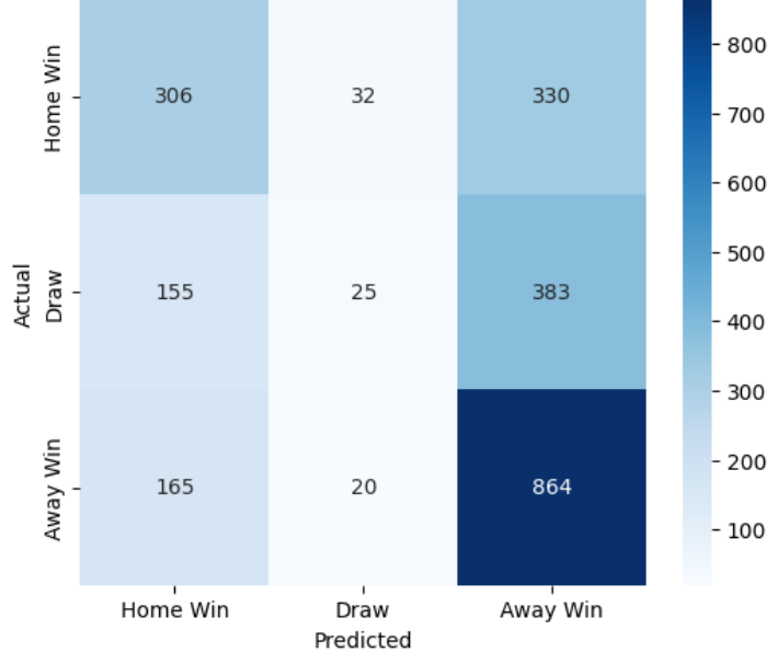
Home Win and Away Win are predicted reasonably well. Draws are almost never predicted correctly — the model collapses most of them into Home Win or Away Win. Final accuracy: ~52%.
K-Means Clustering
An unsupervised method, included more for exploration than as a serious contender. We visualised the clusters using PCA to reduce the feature space down to two dimensions:
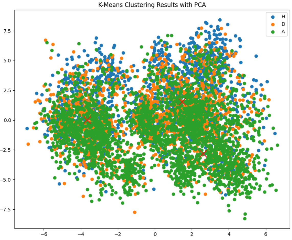
The three cluster centres sit very close together, which explains the low accuracy directly — the classes simply don’t separate cleanly in our feature space. Interestingly, K-Means had the best draw prediction of any model (F1 of 31%), trading overall accuracy for better sensitivity to that harder class. Final accuracy: ~40%.
Results
| Model | Accuracy | Home Win F1 | Away Win F1 | Draw F1 |
|---|---|---|---|---|
| XGBoost | 54% | 0.67 | 0.49 | 0.00 |
| SVM | ~52% | 0.66 | 0.47 | 0.08 |
| DNN | ~50% | 0.62 | 0.50 | 0.15 |
| K-Means | ~40% | 0.42 | 0.45 | 0.31 |
The accuracy vs. draw prediction trade-off was the most interesting finding. XGBoost was clearly the strongest overall, but it completely ignored draws. In the EPL, roughly 25% of matches end level — if you’re building a betting model, blindly ignoring that class will hurt you on certain markets.
The reason draws are hard is intuitive once you think about it: a draw is what happens when neither team dominates. Most features are designed to capture asymmetry between the two sides. When two evenly-matched teams play, the features give the model very little to distinguish between “close, but home team edges it” and “genuinely too close to call.”
Final Predictions
Using XGBoost, our predictions for the 10 February 1st matches:
| Home Team | Away Team | Prediction |
|---|---|---|
| AFC Bournemouth | Liverpool | H |
| Arsenal | Man City | H |
| Brentford | Spurs | H |
| Chelsea | West Ham | H |
| Everton | Leicester City | H |
| Ipswich Town | Southampton | H |
| Man Utd | Crystal Palace | H |
| Newcastle | Fulham | H |
| Nottingham Forest | Brighton | A |
| Wolves | Aston Villa | H |
Nine home wins and one away win. The model heavily favoured home teams — which reflects both the real home advantage in football and the fact that most of our environmental features (travel fatigue, attendance, match density) naturally bode better for the home side. Nottingham Forest vs Brighton is the lone exception, where Brighton’s form and valuation features outweighed the home advantage.
What I’d Do Differently
Ensemble the models. The obvious next step is combining XGBoost’s decisiveness with the draw-sensitivity of K-Means or DNN using stacking or voting. You’d hope to get the best of both without sacrificing either.
Player-level data. Everything we used was team-level. Injuries, suspensions, and individual form matter enormously and aren’t captured at all. A suspended key defender before a big away match is arguably worth several features on its own.
Betting odds as a feature. This sounds circular but it isn’t — bookmaker odds encode a huge amount of market information including injury news, squad selection, and public sentiment. Using odds as an input feature while trying to beat them on accuracy is a legitimate and widely-used approach.
Recency weighting. Our rolling windows treated all matches equally within the window. A loss last week probably matters more than a loss 10 matches ago, and exponential decay weighting would be a natural improvement.
This was one of the more satisfying pieces of coursework from my time at UCL — it sat at the intersection of data engineering, feature design, and model comparison in a way that felt genuinely applied. Football is also a domain where intuition can meaningfully guide feature selection, which made the EDA phase more interesting than usual. The draw prediction problem in particular is something I’d like to revisit properly someday.