Designing a Water-Gas Shift Reactor from Scratch
A UCL final-year project where I modelled, optimised, and stress-tested a high-temperature catalytic reactor for syngas processing — in Python, from the ground up.
For my final-year unit design project at UCL, I designed and optimised a water-gas shift (WGS) reactor for a dimethyl ether (DME) production plant. The deliverable was a complete engineering design — reactor geometry, catalyst specification, operating conditions — backed by a mathematical model built from scratch in Python.
The WGS reaction is CO + H₂O ⇌ CO₂ + H₂. It’s been industrially relevant since the Haber-Bosch era, and it’s still used today in methanol synthesis, Fischer-Tropsch, and hydrogen production to adjust syngas composition. In this context, it sits upstream of a methanol reactor, and its job is to shift the H₂/CO ratio from around 1.41 to something closer to 2 or higher — the sweet spot for methanol synthesis.
The reaction sounds simple. The design problem is not.
The full code is on GitHub.
Why You Can’t Just Run It Adiabatically
The WGS reaction is moderately exothermic at −41.1 kJ/mol. My first instinct — and the simplest design — was to run the reactor adiabatically and let the temperature rise do what it will. So before building the full model, I ran the adiabatic energy balance just to see what happens.
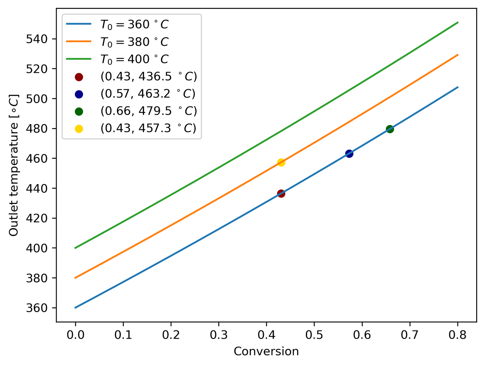
The problem is immediately obvious. Even at a modest inlet of 360°C, the outlet temperature for 80% conversion rockets past 450°C — the point where the Fe-Cr catalyst starts sintering irreversibly. The WGS reaction is also equilibrium-limited, meaning high temperatures actively work against you by pulling the equilibrium constant down. Adiabatic operation is essentially a self-defeating proposition here: the heat released by the reaction undermines the conversion you’re trying to achieve.
The design therefore had to include active cooling. I went with a multi-tubular fixed-bed reactor — catalyst packed inside tubes, coolant flowing in the shell — which is exactly what industrial HT WGS units use. This gives you continuous temperature control along the reactor length rather than managing hot spots by other means.
Building the Model
The reactor is modelled as a 1D pseudohomogeneous system: no radial gradients, plug flow, one representative tube scaled to the full reactor by the number of tubes. I justified each of those assumptions — the Reynolds number (~12,000) confirms turbulent flow, and a quick axial Péclet number check confirmed dispersion is negligible.
The core of the model is a system of ODEs integrated over catalyst weight W:
Mole balance — one ODE per species (CO, H₂O, H₂, CO₂, N₂, CH₄), derived from a differential element of catalyst:
Energy balance — tube temperature coupled to countercurrent coolant:
Pressure drop — Ergun equation adapted to weight-based coordinates.
The rate expression is a Langmuir-Hinshelwood model from Twigg’s Catalyst Handbook, which accounts for adsorption of CO, H₂O, and CO₂ on active sites. Every parameter in the denominator has a temperature dependence, so the rate varies throughout the reactor as conditions shift.
The Effectiveness Factor Problem
Here’s where things got interesting. The WGS reaction on iron-based catalysts is severely diffusion-limited inside the catalyst pellets — reactants have to diffuse into the pores to reach active sites, and that process is slow. To quantify this, I calculated the Thiele modulus Φ₁ for the catalyst particles.
Using Twigg’s reported pre-exponential factor k₀ directly, I got Φ₁ ≈ 111 and η ≈ 0.03. But Twigg himself reports η ≈ 0.96 for similar conditions. Something was off by roughly three orders of magnitude, which is a known issue: the reported k values in the literature likely already embed significant mass transfer effects from the experimental setup used to measure them. Using a naively large k₀ in a model that separately calculates diffusion limitations ends up double-counting the resistance.
The fix was to scale k₀ down by three orders of magnitude, which brought η up to ~0.80 and matched Twigg’s reported range. The effectiveness factor was then baked into the rate constant directly (k := η·k), keeping the pseudohomogeneous model intact.
Optimisation
With the model working, the next step was finding the optimal reactor geometry and operating conditions. I framed this as a minimisation problem: minimise total catalyst weight W subject to hitting 80% CO conversion, while keeping the outlet temperature below 450°C, the pressure drop below 2 bar, and the bed geometry within practical limits.
Five design variables: tube diameter dₜ, number of tubes nₜᵤᵦₑₛ, inlet pressure P₀, inlet temperature T₀, and catalyst particle diameter dₚ. The objective function is non-convex, so I used SciPy’s differential_evolution to search the design space globally.
The optimal solution:
| Parameter | Value |
|---|---|
| Tube diameter | 16.3 mm |
| Number of tubes | 998 |
| Inlet temperature | 360.9°C |
| Inlet pressure | 30.3 bar |
| Particle diameter | 4.0 mm |
| Catalyst weight | 175 kg |
| Reactor volume | 162 L |
The Reactor in Action
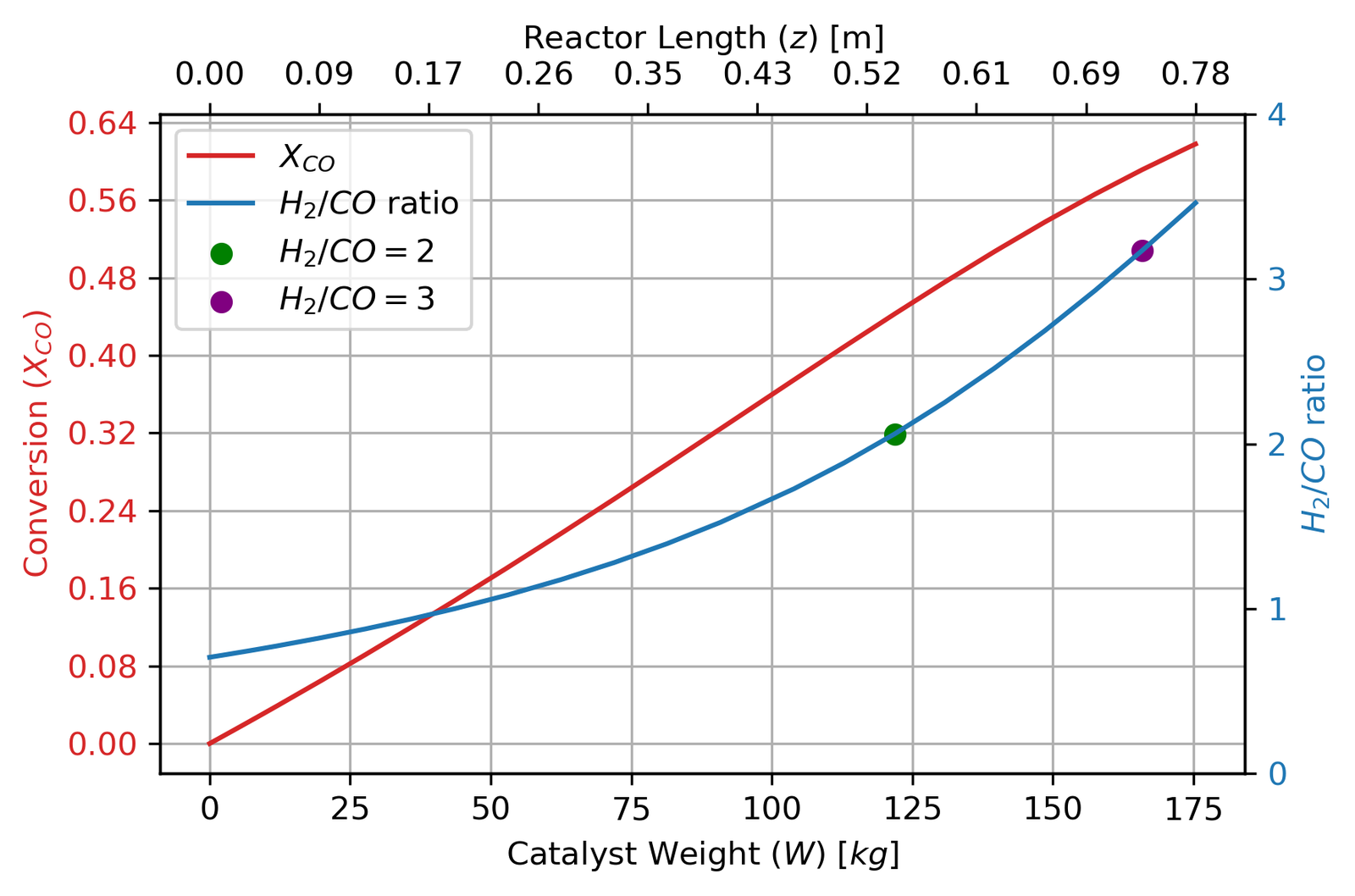
Running the model with these parameters gives the following profiles:
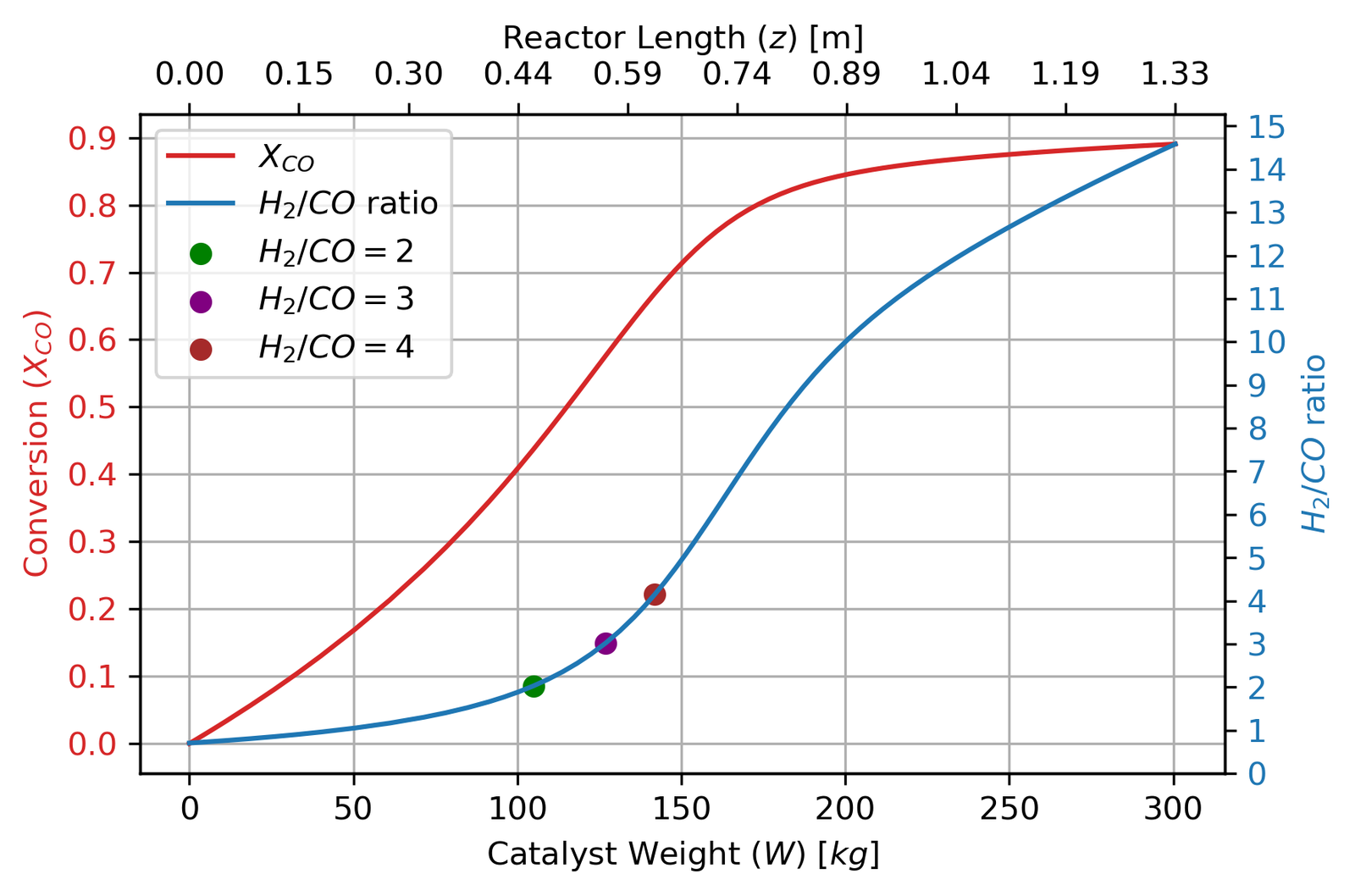
The conversion curve is characteristic of an equilibrium-limited reaction: fast initially, then decelerating sharply as the driving force for reaction (the term [CO][H₂O] − [CO₂][H₂]/K_eq) collapses. By the time the reactor hits 80% conversion at 175 kg, this driving force has dropped by more than an order of magnitude compared to the inlet. The three dots mark H₂/CO ratios of 2, 3, and 4 — useful reference points since downstream methanol synthesis operates best around H₂/CO = 2 to 3.5.
The temperature profile tells the thermal management story:
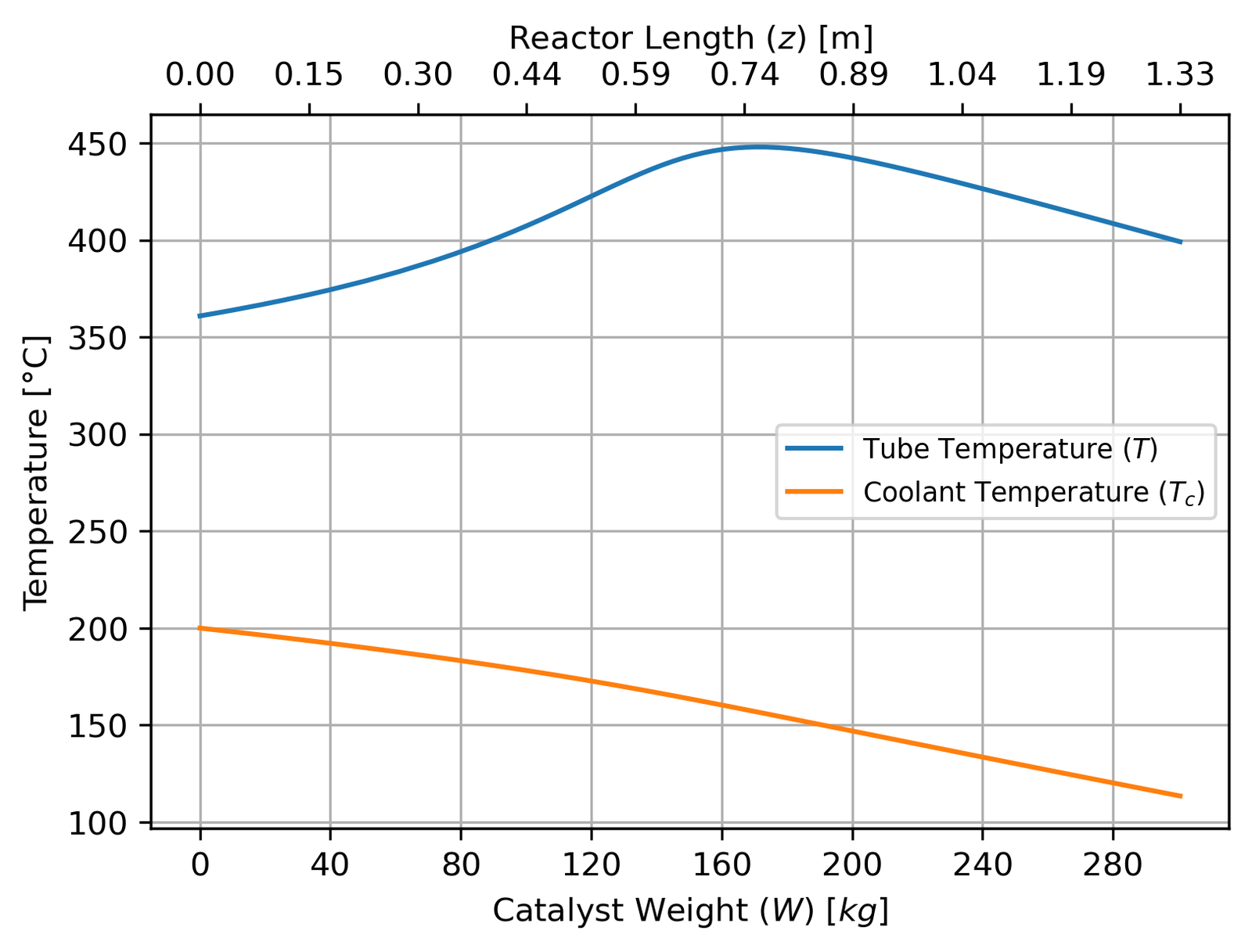
The tube temperature peaks early in the reactor where reaction rates are highest, then falls as the reaction slows down and cooling overtakes heat generation. The coolant enters at 155°C (at the outlet end, since it’s countercurrent) and exits at 200°C — a cooling duty of about 756 kW. The fact that the tube temperature doesn’t monotonically decrease is worth noting: you actually want some of that early temperature rise, because the higher temperature accelerates the kinetics before equilibrium limitations kick in.
Parametric Study
Once the reactor was designed, I fixed the catalyst weight at 175 kg and ran two sets of parametric analyses to understand how sensitive the design is to operating conditions.
Temperature and Pressure
The first study swept inlet temperature T₀ and pressure P₀ over their allowable ranges, recording conversion and outlet temperature simultaneously. I made a 3D plot that encodes three variables at once — T₀, P₀, and X_CO on the axes, with T_out as a colour map:
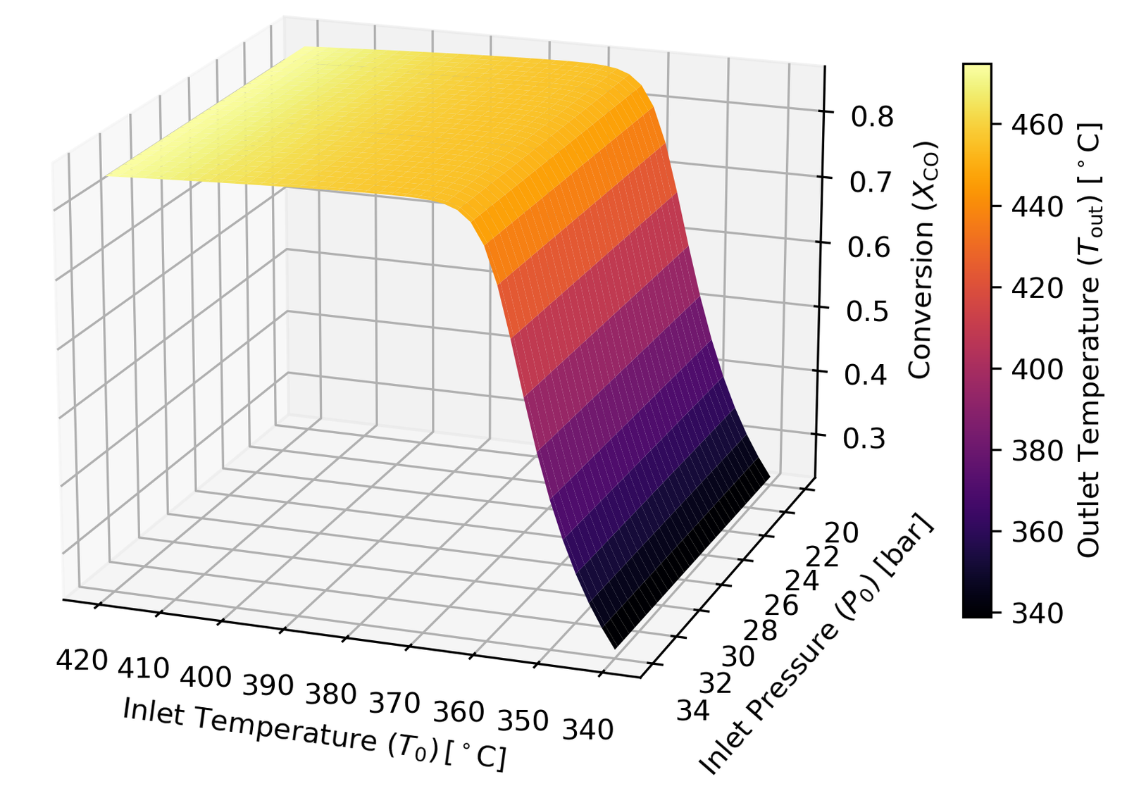
A few things stand out. Below 360°C, conversion falls off sharply — this is where the reaction kinetics slow down enough to also compromise selectivity (the methanation side reaction becomes more competitive). Between 360°C and 390°C, conversion improves modestly but the outlet temperature creeps up. Above 390°C, the equilibrium limitation kicks in hard and conversion gains become negligible, while Tout risks exceeding 450°C and sintering the catalyst. The conclusion: 360–390°C is your operating window, and 361°C specifically is optimal.
Pressure mostly affects the pressure drop rather than conversion directly.
Particle Size
The second study varied the catalyst particle diameter from 1 mm to 10 mm, which is more interesting than it first appears:
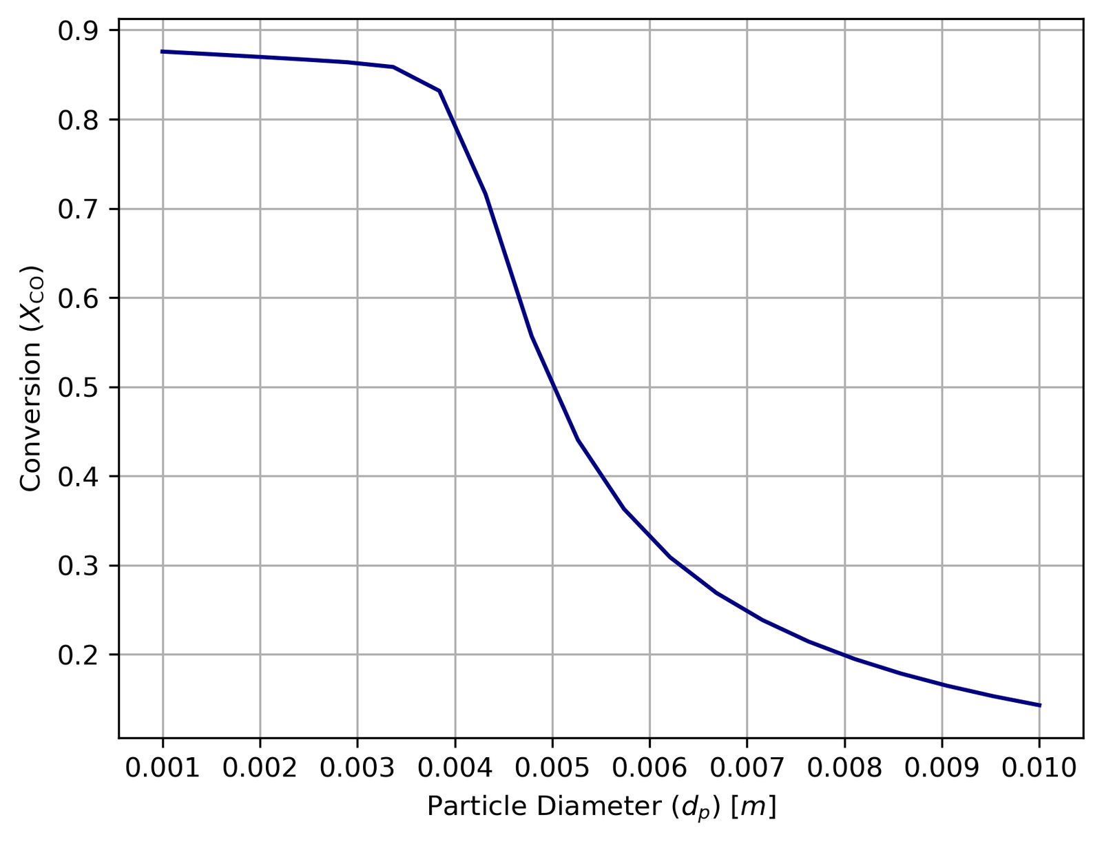
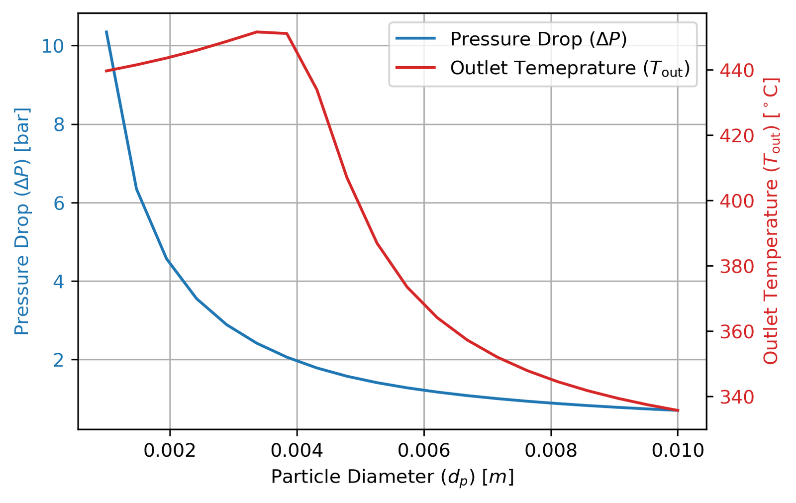
Smaller particles mean better internal diffusion (higher η) and higher conversion. But smaller particles also pack more tightly, creating much higher pressure drops via the Ergun equation. The optimum at 4 mm is precisely the point where conversion is maximised without pushing pressure drop past 2 bar.
The outlet temperature curve has a subtler shape worth explaining: it initially rises as particle size increases before falling. At smaller dp, lower pressure drop means reactant partial pressures stay higher along the entire reactor, concentrating reaction activity near the inlet and producing more heat. Past around 4 mm, the declining η starts to dominate and reaction rates drop everywhere, cooling the outlet. This is a good example of competing effects that aren’t obvious until you actually model them.
What Happens When the Catalyst Ages
Fe-Cr catalysts degrade over time through thermal sintering — iron crystallites grow, blocking active surface area. I modelled a 25% activity loss (realistic for a 3-year operating cycle) by reducing η by 25%.
At the original T₀ = 360°C, conversion drops from 80% to just 45%. Compensating by raising T₀ to 412°C recovers it to about 60% — still enough for methanol synthesis (H₂/CO ≈ 3.5 is acceptable), but not the original 80%.
This is actually how industrial HT WGS reactors are operated in practice: the inlet temperature is gradually nudged upward over the catalyst’s life to compensate for deactivation, right up until Tout hits the sintering threshold and the catalyst has to be replaced. Twigg recommends exactly this approach.
Results Summary
| Metric | Value |
|---|---|
| CO conversion | 80% |
| Outlet temperature | 447°C |
| Pressure drop | ~2 bar |
| Cooling duty | 756 kW |
| Reactor volume | 162 L |
| Catalyst weight | 175 kg |
| Catalyst life | ~3 years |
| Safe operating window | T₀: 360–390°C, P₀: 30–31 bar |
What I’d Do Differently
Get proper kinetic data. The pre-exponential factor k₀ issue was the biggest uncertainty in the whole model. The discrepancy between the raw Twigg data and the calculated Thiele modulus points to a systematic issue with how those rate constants were measured — they were almost certainly determined on packed beds where external and internal mass transfer effects were partially embedded in the reported values. Fitting k₀ to dedicated intrinsic kinetic measurements (differential reactor, crushed catalyst, low conversion) would remove that ambiguity entirely.
Model catalyst deactivation properly. Right now I’m just scaling η by a fixed scalar. A real deactivation model would couple a sintering rate equation to the temperature profile along the reactor — the catalyst near the inlet sees the highest temperature and degrades fastest, which means the activity profile along the reactor changes non-uniformly over time. This would probably predict a faster performance decline than the uniform model suggests.
Validate U experimentally. The overall heat transfer coefficient is fixed at 85 W/m²K from literature. I derived a methodology for estimating U from first principles in an appendix, but it overestimated the value compared to industrial data. U has a direct impact on how well the energy balance holds — if it’s wrong, the temperature profiles are wrong, and the conversion predictions follow.
Consider a two-stage design. For conversions above ~85%, the equilibrium limitation in the HT stage becomes crippling. The industrial solution is a two-stage system: HT WGS for the bulk of the conversion, followed by a smaller LT WGS reactor (copper catalyst, ~200°C) to push conversion higher. For the 43–80% range needed in this plant it’s overkill, but it’s the natural next step if the downstream methanol reactor demanded a higher H₂/CO ratio.
This was one of the more satisfying projects from my time at UCL. Chemical engineering design problems are genuinely constrained optimisation problems — every decision about geometry, operating conditions, or catalyst specification cascades through the physics in multiple directions at once, and the model has to hold it all together. The equilibrium-kinetics-pressure-drop trade-off in particular is one of those things that only clicks once you’ve actually run the numbers.
The full code and report are on GitHub.